Working With NWB Files

from pathlib import Path
import json

import numpy as np
import pandas as pd

from allensdk.brain_observatory.ecephys.ecephys_project_cache import EcephysProjectCache
from allensdk.brain_observatory.ecephys.ecephys_session import EcephysSession

from allensdk.brain_observatory.ecephys import nwb  # for compat
import pynwb
from pynwb import NWBHDF5IO

import nems
from nems0.recording import Recording
from nems0.signal import PointProcess

import h5py

from matplotlib import pyplot as plt

[nems.configs.defaults INFO] Saving log messages to /tmp/nems/NEMS 2019-12-10 155251.log

Generate session and get metadata

data_dir = Path(r'data')
manifest_path = data_dir / 'manifest.json'

manifest.json is where the library keeps a record of previously downloaded files. If it doesn’t exists in location you specify, it will be created the first time you create the cache object. Otherwise, when you request data, the library will check the manifest to see if it’s been downloaded.

# assert manifest_path.exists()

cache = EcephysProjectCache.from_warehouse(manifest=manifest_path)
sessions = cache.get_session_table()

[call_caching INFO] Reading data from cache
[call_caching INFO] Reading data from cache
[call_caching INFO] Reading data from cache
[call_caching INFO] Reading data from cache
[call_caching INFO] Reading data from cache
[numexpr.utils INFO] NumExpr defaulting to 8 threads.
[call_caching INFO] Reading data from cache
[call_caching INFO] Reading data from cache
[call_caching INFO] Reading data from cache
[call_caching INFO] Reading data from cache
[call_caching INFO] Reading data from cache
[call_caching INFO] Reading data from cache
[call_caching INFO] Reading data from cache
[call_caching INFO] Reading data from cache

Download data from session

You can edit the download criteria to filter out the data. Downloading the data can take several minutes.

# 21 is just a random number, for this example notebook
session = cache.get_session_data(sessions.iloc[21].name,
                                 isi_violations_maximum=np.inf,
                                 amplitude_cutoff_maximum=np.inf,
                                 presence_ratio_minimum=-np.inf
                                )

[call_caching INFO] Reading data from cache
[call_caching INFO] Reading data from cache
[call_caching INFO] Reading data from cache
[call_caching INFO] Reading data from cache
[call_caching INFO] Reading data from cache
[call_caching INFO] Reading data from cache
[call_caching INFO] Reading data from cache
[call_caching INFO] Reading data from cache
[call_caching INFO] Reading data from cache
[call_caching INFO] Reading data from cache
[call_caching INFO] Reading data from cache
[call_caching INFO] Reading data from cache
[call_caching INFO] Reading data from cache

This is the epochs table. It applies to all the units.

# this can be slow depending on the size of the data
presentation_table = session.stimulus_presentations
presentation_table.head()

	color	contrast	frame	orientation	phase	pos	size	spatial_frequency	start_time	stimulus_block	stimulus_name	stop_time	temporal_frequency	x_position	y_position	duration	stimulus_condition_id
stimulus_presentation_id
0	null	null	null	null	null	null	null	null	24.752216	null	spontaneous	84.818986	null	null	null	60.066770	0
1	null	0.8	null	45	[3644.93333333, 3644.93333333]	[-30.0, 40.0]	[20.0, 20.0]	0.08	84.818986	0	gabors	85.052505	4	0	10	0.233520	1
2	null	0.8	null	0	[3644.93333333, 3644.93333333]	[-30.0, 40.0]	[20.0, 20.0]	0.08	85.052505	0	gabors	85.302704	4	20	40	0.250199	2
3	null	0.8	null	0	[3644.93333333, 3644.93333333]	[-30.0, 40.0]	[20.0, 20.0]	0.08	85.302704	0	gabors	85.552904	4	-40	40	0.250199	3
4	null	0.8	null	90	[3644.93333333, 3644.93333333]	[-30.0, 40.0]	[20.0, 20.0]	0.08	85.552904	0	gabors	85.803103	4	10	30	0.250199	4

Included is metadata about each unit, as a pandas dataframe.

session.units.head()

[call_caching INFO] Reading data from cache
[call_caching INFO] Reading data from cache
[call_caching INFO] Reading data from cache
[call_caching INFO] Reading data from cache
[call_caching INFO] Reading data from cache
[call_caching INFO] Reading data from cache
[call_caching INFO] Reading data from cache
[call_caching INFO] Reading data from cache
[call_caching INFO] Reading data from cache
[call_caching INFO] Reading data from cache
[call_caching INFO] Reading data from cache
[call_caching INFO] Reading data from cache
[call_caching INFO] Reading data from cache
[call_caching INFO] Reading data from cache
[call_caching INFO] Reading data from cache

	waveform_duration	firing_rate	waveform_PT_ratio	d_prime	waveform_recovery_slope	waveform_velocity_below	presence_ratio	L_ratio	waveform_amplitude	max_drift	...	ecephys_structure_id	ecephys_structure_acronym	anterior_posterior_ccf_coordinate	dorsal_ventral_ccf_coordinate	left_right_ccf_coordinate	probe_description	location	probe_sampling_rate	probe_lfp_sampling_rate	probe_has_lfp_data
unit_id
951853174	0.219765	19.441146	0.199007	6.714259	-0.049973	0.206030	0.99	0.000089	84.471855	48.84	...	215.0	APN	7928	3129	7167	probeA		29999.96621	1249.998592	True
951853190	0.137353	10.267881	0.734993	2.744475	-0.154760	-0.431682	0.99	0.137435	95.045925	50.17	...	215.0	APN	7908	3068	7169	probeA		29999.96621	1249.998592	True
951853197	0.151089	10.161642	0.625356	3.389818	-0.102740	-0.343384	0.99	0.073114	73.191495	47.14	...	215.0	APN	7905	3060	7169	probeA		29999.96621	1249.998592	True
951853216	0.563149	6.664585	0.645313	5.647242	-0.024678	0.286153	0.99	0.009056	45.769815	32.12	...	215.0	APN	7866	2948	7168	probeA		29999.96621	1249.998592	True
951853225	0.576884	9.174408	0.558268	4.388771	-0.033880	0.073582	0.99	0.017206	57.620160	38.75	...	215.0	APN	7854	2913	7167	probeA		29999.96621	1249.998592	True

5 rows × 89 columns

Spike times are stored in a dictionary, with the unit IDs as keys and arrays for the spike times.

# this is a large dict, so let's just look at one key
session.spike_times[951853174]

[call_caching INFO] Reading data from cache
[call_caching INFO] Reading data from cache
[call_caching INFO] Reading data from cache
[call_caching INFO] Reading data from cache
[call_caching INFO] Reading data from cache
[call_caching INFO] Reading data from cache
[call_caching INFO] Reading data from cache

array([3.79479685e+00, 3.80853020e+00, 3.80933020e+00, ...,
       9.62280203e+03, 9.62339993e+03, 9.62352627e+03])

Loading existing NWB files with session

If you’ve previously downloaded data, you can avoid the cache creation and just create a session from an NWB file.

nwb_filepath = Path(r'/auto/users/tomlinsa/code/allen/data/session_760345702/session_760345702.nwb')
assert nwb_filepath.exists()

session = EcephysSession.from_nwb_path(str(nwb_filepath), api_kwargs={
        "amplitude_cutoff_maximum": np.inf,
        "presence_ratio_minimum": -np.inf,
        "isi_violations_maximum": np.inf
    })

# session.stimulus_presentations

or from NWB file (preffered)

This is the raw data. The session method of getting the data does it’s own formatting of the dataframes.

nwb_filepath = Path(r'/auto/users/tomlinsa/code/allen/data/session_760345702/session_760345702.nwb')
assert nwb_filepath.exists()

io = NWBHDF5IO(str(nwb_filepath), 'r')
nwbfile = io.read()

nwbfile.lab_meta_data

{'metadata':
 metadata <class 'allensdk.brain_observatory.ecephys.nwb.EcephysLabMetaData'>
 Fields:
   age_in_days: 103.0
   full_genotype: Pvalb-IRES-Cre/wt;Ai32(RCL-ChR2(H134R)_EYFP)/wt
   sex: M
   specimen_name: Pvalb-IRES-Cre;Ai32-407972
   stimulus_name: brain_observatory_1.1
   strain: C57BL/6J}

The rest of the attributes are still accessible.

# nwbfile.units
# nwbfile.epochs
# nwbfile.stimulus_presentations

Load into NEMS

r = Recording.from_nwb(nwb_filepath, 'neuropixel')

[nems.recording INFO] Loading NWB file with format "neuropixel" from "/auto/users/tomlinsa/code/allen/data/session_760345702/session_760345702.nwb".
[nems.recording INFO] Successfully loaded nwb file.

All of the usual attributes are accessible.

r.epochs.head()

	start	end	name	stimulus_block	temporal_frequency	x_position	y_position	color	colorSpace	depth	...	tex	texRes	units	stimulus_index	orientation	spatial_frequency	frame	contrast	flipHoriz	flipVert
0	24.752216	84.818986	spontaneous	NaN	NaN	NaN	NaN			NaN	...		NaN		NaN	NaN		NaN	NaN	NaN	NaN
1	84.818986	85.052505	gabors	0.0	4.0	0.0	10.0	[1.0, 1.0, 1.0]	rgb	0.0	...	sin	256.0	deg	0.0	45.0	0.08	NaN	0.8	NaN	NaN
2	85.052505	85.302704	gabors	0.0	4.0	20.0	40.0	[1.0, 1.0, 1.0]	rgb	0.0	...	sin	256.0	deg	0.0	0.0	0.08	NaN	0.8	NaN	NaN
3	85.302704	85.552904	gabors	0.0	4.0	-40.0	40.0	[1.0, 1.0, 1.0]	rgb	0.0	...	sin	256.0	deg	0.0	0.0	0.08	NaN	0.8	NaN	NaN
4	85.552904	85.803103	gabors	0.0	4.0	10.0	30.0	[1.0, 1.0, 1.0]	rgb	0.0	...	sin	256.0	deg	0.0	90.0	0.08	NaN	0.8	NaN	NaN

5 rows × 27 columns

r.meta

{'specimen_name': 'Pvalb-IRES-Cre;Ai32-407972',
 'age_in_days': 103.0,
 'full_genotype': 'Pvalb-IRES-Cre/wt;Ai32(RCL-ChR2(H134R)_EYFP)/wt',
 'strain': 'C57BL/6J',
 'sex': 'M',
 'stimulus_name': 'brain_observatory_1.1',
 'uri': '/auto/users/tomlinsa/code/allen/data/session_760345702/session_760345702.nwb'}

All of the spike times are saved into a single PointProcess signal.

r.signals

{'session_760345702': <nems.signal.PointProcess at 0x7fd3ea723f98>}

signal = r.signals['session_760345702']
signal.nchans

1784

Each channel key is the unit ID from the units dataframe of the NWB file

# ex, unit 951843010
signal._data[951843010]

array([  10.2351168 ,   11.66955413,   11.69268753, ..., 9612.18553725,
       9612.20010396, 9620.83476135])

The units metadata is saved into the meta of the signal.

# ex, unit 951843010
signal.meta[951843010]

{'waveform_duration': 0.755443886097152,
 'firing_rate': 1.74113707219344,
 'PT_ratio': 0.00729943086142739,
 'd_prime': nan,
 'recovery_slope': -0.00895206089461061,
 'quality': 'noise',
 'velocity_below': 1.03015075376884,
 'presence_ratio': 0.99,
 'l_ratio': 0.0,
 'amplitude': 51.4938450000001,
 'max_drift': 23.6,
 'snr': 1.92770330724404,
 'nn_hit_rate': nan,
 'spread': 60.0,
 'nn_miss_rate': nan,
 'cumulative_drift': 615.49,
 'waveform_halfwidth': 0.357118927973199,
 'isolation_distance': nan,
 'isi_violations': 1.06689648479891,
 'silhouette_score': 0.0759991877886951,
 'local_index': 263,
 'amplitude_cutoff': 0.268061054461112,
 'repolarization_slope': 0.122863156143529,
 'cluster_id': 267,
 'velocity_above': 1.37353433835846,
 'peak_channel_id': 850096152}

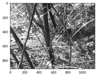
Get stimulus images

For example, frame 100 from natural_scenes, as in this random row:

r.epochs.loc[[51357], ['start', 'end', 'name', 'frame']]  # list loc to keep as df

	start	end	name	frame
51357	5910.169789	5910.420001	natural_scenes	100.0

im = cache.get_natural_scene_template(100)

[call_caching INFO] Reading data from cache

plt.imshow(im, cmap=plt.cm.gray)

<matplotlib.image.AxesImage at 0x7fd3ea60bf60>